In this blog post, I am going to go through as series of neural network structures. This is intended as a demonstration of the more basic neural net functionality. This blog post serves as an accompanyment to the introduction to machine learning chapter of the short book I am writing ( Currently under the working title “Neural Network Representations for Natural Language Processing”)
I do have an earlier blog covering some similar topics. However, I exect the code in this one to be a lot more sensible, since I am now much more familar with TensorFlow.jl, having now written a significant chunk of it. Also MLDataUtils.jl is in different state to what it was.
Input:
using TensorFlow
using MLDataUtils
using MLDatasets

using ProgressMeter

using Base.Test
using Plots
gr()
using FileIO
using ImageCore
MNIST classifier
This is the most common benchmark for neural network classifiers. MNIST is a collection of hand written digits from 0 to 9. The task is to determine which digit is being shown. With neural networks this is done by flattening the images into vectors, and using one-hot encoded outputs with softmax.
Input:
"""Makes 1 hot, row encoded labels."""
onehot_encode_labels(labels_raw) = convertlabel(LabelEnc.OneOfK, labels_raw, LabelEnc.NativeLabels(collect(0:9)),  LearnBase.ObsDim.First())
"""Convert 3D matrix of row,column,observation to vector,observation"""
flatten_images(img_raw) = squeeze(mapslices(vec, img_raw,1:2),2)


@testset "data prep" begin
    @test onehot_encode_labels([4,1,2,3,0]) == [0 0 0 0 1 0 0 0 0 0
                                  0 1 0 0 0 0 0 0 0 0
                                  0 0 1 0 0 0 0 0 0 0
                                  0 0 0 1 0 0 0 0 0 0
                                  1 0 0 0 0 0 0 0 0 0]

    data_b1 = flatten_images(MNIST.traintensor())
    @test size(data_b1) == (28*28, 60_000)
    labels_b1 = onehot_encode_labels(MNIST.trainlabels())
    @test size(labels_b1) == (60_000, 10)
end;
Output:
Test Summary: | Pass  Total
data prep     |    3      3
A visualisation of one of the examples from MNIST. Code is a little complex because of the unflattening, and adding a border.
Input:
const frames_image_res = 30

"Convests a image vector into a framed 2D image"
function one_image(img::Vector)
    ret = zeros((frames_image_res, frames_image_res))
    ret[2:end-1, 2:end-1] = 1-rotl90(reshape(img, (28,28)))
    ret
end

train_images=flatten_images(MNIST.traintensor())
heatmap(one_image(train_images[:,10]))
Output:
<?xml version=”1.0” encoding=”utf-8”?>
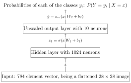
In this basic example we use a traditional sigmoid feed-forward neural net. It uses just a single wide hidden layer. It works surprisingly well compaired to early benchmarks. This is becuase the layer is very wide compaired to what was possible 30 years ago.
Input:
load("Intro\ to\ Machine\ Learning\ with\ Tensorflow.jl/mnist-basic.png")Output:

Input:
sess = Session(Graph())
@tf begin
    X = placeholder(Float32, shape=[-1, 28*28])
    Y = placeholder(Float32, shape=[-1, 10])

    W1 = get_variable([28*28, 1024], Float32)
    b1 = get_variable([1024], Float32)
    Z1 = nn.sigmoid(X*W1 + b1)

    W2 = get_variable([1024, 10], Float32)
    b2 = get_variable([10], Float32)
    Z2 = Z1*W2 + b2 # Affine layer on its own, to get the unscaled logits
    Y_probs = nn.softmax(Z2)

    losses = nn.softmax_cross_entropy_with_logits(;logits=Z2, labels=Y) #This loss function takes the unscaled logits
    loss = reduce_mean(losses)
    optimizer = train.minimize(train.AdamOptimizer(), loss)
end
Output:
2017-08-02 18:53:18.598588: W tensorflow/core/platform/cpu_feature_guard.cc:45] The TensorFlow library wasn't compiled to use SSE4.1 instructions, but these are available on your machine and could speed up CPU computations.
2017-08-02 18:53:18.598620: W tensorflow/core/platform/cpu_feature_guard.cc:45] The TensorFlow library wasn't compiled to use SSE4.2 instructions, but these are available on your machine and could speed up CPU computations.
2017-08-02 18:53:18.598626: W tensorflow/core/platform/cpu_feature_guard.cc:45] The TensorFlow library wasn't compiled to use AVX instructions, but these are available on your machine and could speed up CPU computations.
2017-08-02 18:53:18.789486: I tensorflow/stream_executor/cuda/cuda_gpu_executor.cc:893] successful NUMA node read from SysFS had negative value (-1), but there must be at least one NUMA node, so returning NUMA node zero
2017-08-02 18:53:18.789997: I tensorflow/core/common_runtime/gpu/gpu_device.cc:940] Found device 0 with properties:
name: GeForce GTX TITAN X
major: 5 minor: 2 memoryClockRate (GHz) 1.076
pciBusID 0000:01:00.0
Total memory: 11.91GiB
Free memory: 11.42GiB
2017-08-02 18:53:18.790010: I tensorflow/core/common_runtime/gpu/gpu_device.cc:961] DMA: 0
2017-08-02 18:53:18.790016: I tensorflow/core/common_runtime/gpu/gpu_device.cc:971] 0:   Y
2017-08-02 18:53:18.790027: I tensorflow/core/common_runtime/gpu/gpu_device.cc:1030] Creating TensorFlow device (/gpu:0) -> (device: 0, name: GeForce GTX TITAN X, pci bus id: 0000:01:00.0)
<Tensor Group:1 shape=unknown dtype=Any>
Train
We use normal minibatch training with Adam.
We do use relatively large minibatches, as that gets best performance advantage on GPU,
by minimizing memory transfers.
A more advanced implementation might do a the batching within Tensorflow,
rather than batching outside tensorflow and invoking it via run.
Input:
traindata = (flatten_images(MNIST.traintensor()), onehot_encode_labels(MNIST.trainlabels()))
run(sess, global_variables_initializer())


basic_train_loss = Float64[]
@showprogress for epoch in 1:100
    epoch_loss = Float64[]
    for (batch_x, batch_y) in eachbatch(traindata, 1000, (ObsDim.Last(), ObsDim.First()))
        loss_o, _ = run(sess, (loss, optimizer), Dict(X=>batch_x', Y=>batch_y))
        push!(epoch_loss, loss_o)
    end
    push!(basic_train_loss, mean(epoch_loss))
    #println("Epoch $epoch: $(train_loss[end])")
end
Output:
Progress: 100%|█████████████████████████████████████████| Time: 0:01:25Input:
plot(basic_train_loss, label="training loss")Output:
<?xml version=”1.0” encoding=”utf-8”?>
Test
Input:
testdata_x = flatten_images(MNIST.testtensor())
testdata_y = onehot_encode_labels(MNIST.testlabels())

y_probs_o = run(sess, Y_probs, Dict(X=>testdata_x'))
acc = mean(mapslices(indmax, testdata_y, 2) .== mapslices(indmax, y_probs_o, 2) )

println("Error Rate: $((1-acc)*100)%")
Output:
Error Rate: 1.9299999999999984%Advanced MNIST classifier
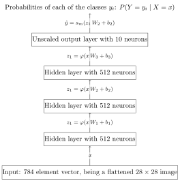
Here we will use more advanced TensorFlow features, like indmax,
and also a more advanced network.
Input:
load("Intro\ to\ Machine\ Learning\ with\ Tensorflow.jl/mnist-advanced.png")Output:

Input:
sess = Session(Graph())

# Network Definition
begin
    X = placeholder(Float32, shape=[-1, 28*28])
    Y = placeholder(Float32, shape=[-1])
    KeepProb = placeholder(Float32, shape=[])

    # Network parameters
    hl_sizes = [512, 512, 512]
    activation_functions = Vector{Function}(size(hl_sizes))
    activation_functions[1:end-1]=z->nn.dropout(nn.relu(z), KeepProb)
    activation_functions[end] = identity #Last function should be idenity as we need the logits

    Zs = [X]
    for (ii,(hlsize, actfun)) in enumerate(zip(hl_sizes, activation_functions))
        Wii = get_variable("W_$ii", [get_shape(Zs[end], 2), hlsize], Float32)
        bii = get_variable("b_$ii", [hlsize], Float32)
        Zii = actfun(Zs[end]*Wii + bii)
        push!(Zs, Zii)
    end

    Y_probs = nn.softmax(Zs[end])
    Y_preds = indmax(Y_probs,2)-1 # Minus 1, to offset 1 based indexing

    losses = nn.sparse_softmax_cross_entropy_with_logits(;logits=Zs[end], labels=Y+1) # Plus 1, to offset 1 based indexing
    #This loss function takes the unscaled logits, and the numerical labels
    loss = reduce_mean(losses)
    optimizer = train.minimize(train.AdamOptimizer(), loss)
end
Output:
2017-08-02 19:27:57.180945: I tensorflow/core/common_runtime/gpu/gpu_device.cc:1030] Creating TensorFlow device (/gpu:0) -> (device: 0, name: GeForce GTX TITAN X, pci bus id: 0000:01:00.0)<Tensor Group:1 shape=unknown dtype=Any>
Train
Input:
traindata_x = flatten_images(MNIST.traintensor())
normer = fit(FeatureNormalizer, traindata_x)
predict!(normer, traindata_x); # perhaps oddly, in current version of MLDataUtils the Normalizer commands to normalize is `predict`

traindata_y = Int.(MNIST.trainlabels());
Input:
run(sess, global_variables_initializer())
adv_train_loss = Float64[]
@showprogress for epoch in 1:100
    epoch_loss = Float64[]
    for (batch_x, batch_y) in eachbatch((traindata_x, traindata_y), 1000, ObsDim.Last())
        loss_o, _ = run(sess, (loss, optimizer), Dict(X=>batch_x', Y=>batch_y, KeepProb=>0.5f0))
        push!(epoch_loss, loss_o)
    end
    push!(adv_train_loss, mean(epoch_loss))
    #println("Epoch $epoch: $(train_loss[end])")
end
Output:
Progress: 100%|█████████████████████████████████████████| Time: 0:01:10Input:
plot([basic_train_loss, adv_train_loss], label=["basic", "advanced"])Output:
<?xml version=”1.0” encoding=”utf-8”?>
Test
Input:
testdata_x = predict!(normer, flatten_images(MNIST.testtensor()))
testdata_y = Int.(MNIST.testlabels());

y_preds_o = run(sess, Y_preds, Dict(X=>testdata_x', KeepProb=>1.0f0))
acc = mean(testdata_y .== y_preds_o )

println("Error Rate: $((1-acc)*100)%")
Output:
Error Rate: 1.770000000000005%It can be seen that overall all the extra stuff done in the advanced model did not gain much. The margin is small enough that it can be attributed to in part to luck – repeating it can do better or worse depending on the random initialisations. Classifying MNIST is perhaps too simpler problem for deep techneques to pay off.
Bottle-necked Autoencoder
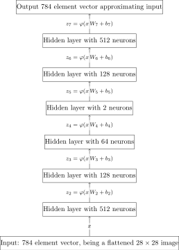
An autoencoder is a neural network designed to recreate its inputs. There are many varieties, include RBMs, DBNs, SDAs, mSDAs, VAEs. This is one of the simplest being based on just a feedforward neural network.
The network narrows into to a very small central layer – in this case just 2 neurons, before exampanding back to the full size. It is sometimes called a Hour-glass, or Wine-glass autoencoder to describe this shape.
Input:
load("Intro\ to\ Machine\ Learning\ with\ Tensorflow.jl/autoencoder.png")Output:

Input:
sess = Session(Graph())

# Network Definition

begin
    X = placeholder(Float32, shape=[-1, 28*28])

    # Network parameters
    hl_sizes = [512, 128, 64, 2, 64, 128, 512, 28*28]
    activation_functions = Vector{Function}(size(hl_sizes))
    activation_functions[1:end-1] = x -> 0.01x + nn.relu6(x)
        # Neither sigmoid, nor relu work anywhere near as well here
        # relu6 works sometimes, but the hidden neurons die too often
        # So we define a leaky ReLU6 as above
    activation_functions[end] = nn.sigmoid #Between 0 and 1


    Zs = [X]
    for (ii,(hlsize, actfun)) in enumerate(zip(hl_sizes, activation_functions))
        Wii = get_variable("W_$ii", [get_shape(Zs[end], 2), hlsize], Float32)
        bii = get_variable("b_$ii", [hlsize], Float32)
        Zii = actfun(Zs[end]*Wii + bii)
        push!(Zs, Zii)
    end


    Z_code = Zs[end÷2 + 1] # A name for the coding layer
    has_died = reduce_any(reduce_all(Z_code.==0f0, axis=2))

    losses = 0.5(Zs[end]-X)^2

    loss = reduce_mean(losses)
    optimizer = train.minimize(train.AdamOptimizer(), loss)
end
Output:
2017-08-02 19:52:56.573001: W tensorflow/core/platform/cpu_feature_guard.cc:45] The TensorFlow library wasn't compiled to use SSE4.1 instructions, but these are available on your machine and could speed up CPU computations.
2017-08-02 19:52:56.573045: W tensorflow/core/platform/cpu_feature_guard.cc:45] The TensorFlow library wasn't compiled to use SSE4.2 instructions, but these are available on your machine and could speed up CPU computations.
2017-08-02 19:52:56.573054: W tensorflow/core/platform/cpu_feature_guard.cc:45] The TensorFlow library wasn't compiled to use AVX instructions, but these are available on your machine and could speed up CPU computations.
2017-08-02 19:52:56.810042: I tensorflow/stream_executor/cuda/cuda_gpu_executor.cc:893] successful NUMA node read from SysFS had negative value (-1), but there must be at least one NUMA node, so returning NUMA node zero
2017-08-02 19:52:56.810561: I tensorflow/core/common_runtime/gpu/gpu_device.cc:940] Found device 0 with properties:
name: GeForce GTX TITAN X
major: 5 minor: 2 memoryClockRate (GHz) 1.076
pciBusID 0000:01:00.0
Total memory: 11.91GiB
Free memory: 11.42GiB
2017-08-02 19:52:56.810575: I tensorflow/core/common_runtime/gpu/gpu_device.cc:961] DMA: 0
2017-08-02 19:52:56.810584: I tensorflow/core/common_runtime/gpu/gpu_device.cc:971] 0:   Y
2017-08-02 19:52:56.810602: I tensorflow/core/common_runtime/gpu/gpu_device.cc:1030] Creating TensorFlow device (/gpu:0) -> (device: 0, name: GeForce GTX TITAN X, pci bus id: 0000:01:00.0)
<Tensor Group:1 shape=unknown dtype=Any>
The choice of activation function here, is (as mentioned in the comments) a bit special. On this particular problem, as a deep network, sigmoid was not going well presumably because of the exploding/vanishing gradient issue that normally cases it to not work out (though I did not check).
Switching to ReLU did not help, though I now suspect I didn’t give it enough tries. ReLU6 worked great the first few tries, but coming back to it later, and I found I couldn’t get it to train because one or both of the hidden units would die, which I did see the first times I trained it but not as commonly.
The trick to make this never happen was to allow the units to turn themselves back on. This is done by providing a non-zero gradient for the off-states. A leaky RELU6 unit. Mathematically it is given by \(\varphi(z)=\begin{cases} 0.01z+6 && 6<z \\ 1.01z && 0 \le z \le 6 \\ 0.01z && z < 0 \end{cases}\)
Training
Input:
train_images = flatten_images(MNIST.traintensor())
test_images = flatten_images(MNIST.testtensor());
Input:
run(sess, global_variables_initializer())
auto_loss = Float64[]
@showprogress for epoch in 1:75
    epoch_loss = Float64[]
    for batch_x in eachbatch(train_images, 1_000, ObsDim.Last())
        loss_o, _ = run(sess, (loss, optimizer), Dict(X=>batch_x'))
        push!(epoch_loss, loss_o)
    end
    push!(auto_loss, mean(epoch_loss))
    #println("Epoch $epoch loss: $(auto_loss[end])")

    ### Check to see if it died
    if run(sess, has_died, Dict(X=>train_images'))
        error("Neuron in hidden layer has died, must reinitialize.")
    end
end
Output:
Progress: 100%|█████████████████████████████████████████| Time: 0:01:51Input:
plot([auto_loss], label="Autoencoder Loss")Output:
<?xml version=”1.0” encoding=”utf-8”?>
Input:
function reconstruct(img::Vector)
    run(sess, Zs[end], Dict(X=>reshape(img, (1,28*28))))[:]
end
Output:
reconstruct (generic function with 1 method)
Input:
id = 120
heatmap([one_image(train_images[:,id]) one_image(reconstruct(train_images[:,id]))])
Output:
<?xml version=”1.0” encoding=”utf-8”?>
Input:
id = 1
heatmap([one_image(test_images[:,id]) one_image(reconstruct(test_images[:,id]))])
Output:
<?xml version=”1.0” encoding=”utf-8”?>
Visualising similarity
One of the key uses of an autoencoder such as this is to project from a the high dimentional space of the inputs, to the low dimentional space of the code layer.
Input:
function scatter_image(images, res)
    canvas = ones(res, res)

    codes = run(sess, Z_code, Dict(X=>images'))
    codes = (codes .- minimum(codes))./(maximum(codes)-minimum(codes))
    @assert(minimum(codes) >= 0.0)
    @assert(maximum(codes) <= 1.0)

    function target_area(code)
        central_res = res-frames_image_res-1
        border_offset = frames_image_res/2 + 1
        x,y = code*central_res + border_offset

        get_pos(v) = round(Int, v-frames_image_res/2)
        x_min = get_pos(x)
        x_max = x_min + frames_image_res-1
        y_min =  get_pos(y)
        y_max = y_min + frames_image_res-1

        @view canvas[x_min:x_max, y_min:y_max]
    end

    for ii in 1:size(codes, 1)
        code = codes[ii,:]
        img = images[:,ii]
        area = target_area(code)
        any(area.<1) && continue # Don't draw over anything
        area[:] = one_image(img)
    end
    canvas
end
heatmap(scatter_image(test_images, 700))
Output:
<?xml version=”1.0” encoding=”utf-8”?>
Input:
heatmap(scatter_image(test_images, 4_000))
savefig("mnist_scatter.pdf")
A high-resolution PDF with more numbers shown can be downloaded from here
So the position of each digit shown on the scatter-plot is given by the level of activation of the coding layer neurons. Which are basically a compressed repressentation of the image.
We can see not only are the images roughly grouped acording to their number, they are also positioned accoridng to appeance. In the top-right it can be seen arrayed are all the ones. With there posistion (seemingly) determined by the slant. Other numbers with similarly slanted potions are positioned near them. The implict repressentation found using the autoencoder unviels hidden properties of the images.
Conclusion
We have presented a few fairly basic neural network models. Hopefully, the techneques shown encourage you to experiment further with machine learning with Julia, and TensorFlow.jl.